Spatiocyte Method
In this section, we summarize the underlying features of the Spatiocyte method that are necessary to build an RD model. For a more detailed description of the method we direct the reader to a previous article (Arjunan and Tomita, 2010).
The Spatiocyte method discretizes the space into a hexagonal close-packed (HCP) lattice of regular sphere voxels with radius rv. Each voxel has 12 adjoining neighbors. To represent a surface compartment such as a cell or a nuclear membrane, all empty voxels of the compartment are occupied with immobile lipid molecules. The method also allows molecules to be simulated at microscopic and compartmental spatial scales simultaneously. In the former, each molecule is discrete and treated individually. For example, each diffusing molecule at the microscopic scale is moved independently by a DiffusionProcess from a source voxel to a target neighbor voxel after a given diffusion step interval. Immobile molecules are also simulated at the microscopic scale. Conversely at the compartmental scale, molecules are assumed to be homogeneously distributed (HD) and thus, the concentration information of each HD species is sufficient without explicit diffusion movements. Depending on the simulated spatial scale and the mobility of the reacting species, molecules can undergo either diffusion-influenced or diffusion-decoupled reactions.
All second-order reactions comprising two diffusing reactants, or a diffusing and an immobile reactant are diffusion-influenced, and are therefore, executed by the DiffusionInfluencedReactionProcess. The remaining reactions, which include all zeroth- and first-order reactions, and second-order reactions that involve two adjoining immobile reactants or at least one HD reactant, can be decoupled from diffusion. These diffusion-decoupled reactions are performed by the SpatiocyteNextReactionProcess.
We proceed with the execution of DiffusionInfluencedReactionProcess for a reaction j. Following our discretized scheme (Arjunan and Tomita, 2010) of the Collins and Kimball RD approach (Collins and Kimball, 1949), when a diffusing molecule collides with a reactant pair of j at the target voxel, they react with probability
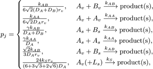
where the constant 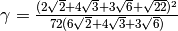 , L is the lipid species, k is the intrinsic
reaction rate of j, D is the diffusion coefficient, while the species
subscripts v and s denote volume and surface species respectively.
, L is the lipid species, k is the intrinsic
reaction rate of j, D is the diffusion coefficient, while the species
subscripts v and s denote volume and surface species respectively.
The DiffusionProcess handles the voxel-to-voxel random walk of diffusing molecules and the collisions that take place between each walk. The latter is necessary when a diffusing species participates in a strongly diffusion-limited reaction and the time slice between each walk is too large for an accurate value of pj. Given ts is the current simulation time, the next time a molecule of a diffusing species i with a diffusion coefficient Di can be moved to a randomly selected neighbor voxel is

where in the HCP lattice, the constant  if it is a volume
species or
if it is a volume
species or 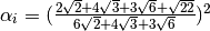 if it belongs to a surface compartment. However, if
i participates in a diffusion-limited reaction, a reactive collision may
take place at time slices smaller than the walk interval
if it belongs to a surface compartment. However, if
i participates in a diffusion-limited reaction, a reactive collision may
take place at time slices smaller than the walk interval  ,
causing pj > 1. To ensure pj ≤ 1, we reduce the DiffusionProcess
interval such that its next execution time becomes
,
causing pj > 1. To ensure pj ≤ 1, we reduce the DiffusionProcess
interval such that its next execution time becomes
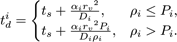
Here Pi is an arbitrarily set reaction probability limit (default value is unity) such that 0 ≤ Pi ≤ 1, and ρi=max{p1, … , pJ} where J is the total number of diffusion-influenced reactions participated by the species i. At each process interval, the molecule can collide as usual with a neighbor reactant pair and react with a scaled probability of pjPi/ρi. In the diffusion-limited case, ρi > Pi and because of the reduced interval, the walk probability becomes less than unity to Pi/ρi.
Reactions that can be decoupled from diffusion such as zeroth- and first-order reactions, and second-order reactions that involve two adjoining immobile reactants or at least one HD reactant, are event-driven by the SpatiocyteNextReactionProcess. The reaction product can be made up of one or two molecules, which can be either HD or nonHD molecules. The SpatiocyteNextReactionProcess is an adapted implementation of the Next Reaction (NR) method (Gibson and Bruck, 2000), which itself is a variation of the Gillespie algorithm (Gillespie 1976, 1977).
In the process, the reaction propensity  (unit s-1) is
calculated from the rate coefficient according to
(unit s-1) is
calculated from the rate coefficient according to
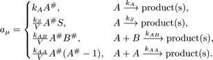
Here, S and V are area and volume of the reaction compartment respectively, while kS (unit ms-1) is the surface-average adsorption rate of an HD volume species A. In the second-order reactions, V is replaced with S if both reactants are in a surface compartment. The next reaction time of a randomly selected molecule in a first order reaction or a pair of molecules in a second-order reaction is given by

with ur a uniformly distributed random number in the range (0,1).
If a reaction has a nonHD product, the new molecule will replace a nonHD reactant in the product compartment. Otherwise if the reaction only involves HD reactants or if the product belongs to a different compartment, the new nonHD molecule will be placed in a random vacant voxel of the product compartment. The placement of a second nonHD product also follows the same procedure. For intercompartmental reactions, a nonHD product will occupy a vacant voxel adjoining both compartments.
Dynamic localization patterns of simulated molecules can be directly compared with experimentally obtained fluorescence microscopy images and videos using the MicroscopyTrackingProcess and the SpatiocyteVisualizer. Together, these modules simulate the microphotography process by recording the trajectory of simulated molecules over the camera exposure time and displaying their spatially localized densities. The MicroscopyTrackingProcess records the number of times the molecules of a species occupy each voxel at diffusion step intervals over the exposure time. The SpatiocyteVisualizer then displays the species color at each voxel with intensity and opacity levels that are directly proportional the voxel occupancy frequency. Colors from different species occupying the same voxel are blended to mimic co-localization patterns observed in multiple-labeling experiments.